ADNet: Action-based Object Tracking using Reinforcement Learning
Introduction
Over the last decade, visual object tracking has been a hot topic. It has been heavily researched for a variety of applications ranging from video surveillance, robotics to virtual and augmented reality. Over the past three years alone, 57 publications presented a variety of deep learning architectures tackling the problem in NIPS, ICCV, ECCV and CVPR [1]. A variety of datasets have been proposed to benchmark these trackers in a standardized manner. A considerable contribution to the visual tracking community was the Visual Object Tracking (VOT) challenge [2]. It was introduced in 2013 as a standardized metric to compare trackers. It also introduces a programming language-agnostic interface through which trackers could integrate and benchmark against the challenge. The VOT precision and robustness metrics are statistically stable; Every classifier is used to track the same video a few times (usually 5 passes) if it is not deterministic. The challenge toolkit then calculates the average and standard deviation of their precision, robustness and performance.
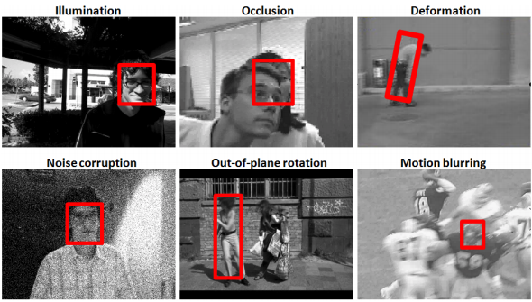
Challengeing appearance changes in visual object tracking resulting from poor illumination, occlusions, out-of-plane rotations, deformations, low-quality sensor data (i.e. noisy images) and motion blurring [3].
Visual trackers face different challenges (see above) like motion blurring, occlusion, out-of-plane rotation, varying lighting conditions, item disappearances between frames, varying input signals (i.e. due to changes in cameras, setup or noise corruption) and small-sized objects [3].
Visual object tracking algorithms often consist of two main components: a feature extractor and a search function. The feature extractor learns distinctive features in each frame. The search function search for these features across each cosecutive frames.
The literature propsed a wide range of solutions to solve the above-mentioned problems. Before deep networks were popular, lots of solutions adopted hand-crafted features to serch for the object or track it across consecutive frames [4], [5], [6], [7], [3], [8], [9], [10]. These solutions were very computationally efficient and ran in realtime. However, given their simplicity and the smaller datasets they trained on, they severely suffered from occlusions and changing lighting conditions.
Recently, with the advancement of deep learning, many convolutional and deep regression networks were proposed [11], [12], [13], [14], [15], [16], [17], [18], [19], [20], [21], [22], [23], [24]. These networks learned a more sophisticated tracking function among consecutive frames and regressed bounding boxes. The regressed bounding boxes varied in each network. Some tracked a bounding box’s center, width and height. Others tracked a bounding box’s upper-left and bottom-right point coordinates. Deep regression networks proved to be a more successful approach as they achieved higher precision, success, and robustness in tracking. However, they were slower than their classical counterparts. With GPU acceleration, some deep regression nets could achieve realtime speeds (i.e. [12]). Despite their accuracy, deep regression networks still suffer severely from occlusion, motion blurring and disappearing objects shortly in some frames.
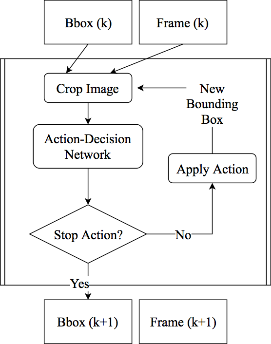
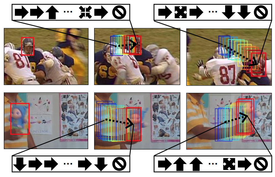
Markov Decision Process: At each frame (\(k\)), we predict an action (\(a_{k,l}\)) using the ADNet. The action is used to obtain a new bounding box (\(b_{k,l}\)). Iteratively, we use the new bounding box to predict the next action in the sequence until we reach a "stop" action (\(a_{k_\mathcal{L}}\)) or a repeated sequence is observed (i.e. left, right, left). Then, we assign \(b_{k,\mathcal{L}}\) to \(b_{k+1}\).
In this paper, we present Action-Decision Networks (ADNets) [25]. ADNets simplify the tracking problem into a sequence of action predictions using a neural network. A pre-trained convolutional network is used as a feature extractor. The network learns to predict a set of actions that would translate into the target’s position.
The authors contributions could be summarized as follows:
- A unique action-based tracking architecture that is more computationally efficient than the deep learning alternatives and achieves satisfactory results.
- First-of-kind semi-supervised deep reinforcement learning for action-based tracking strategy.
- A realtime visual object tracker that outperforms state-of-the-art realtime trackers.
Related Work
In this section, I will touch briefly on some of the existing trackers. Visual object tracking literature could be divided into two clusters: hand-crafted feature-based trackers and deep learning-based trackers. Hand-crafted feature-based trackers often consists of appearance models, point descriptors (i.e. SIFT and SURF), filter-based, and kernel-based features. Hand-crafted trackers often used a tracking-by-detection approach. Deep learning-based trackers use pre-trained convolutional layers to learn a regression function given an object’s original location. The bounding box coordinates are regressed using a fully connected network.
DSST [26] presents a correlation filter-based approach in order to track objects in multiple scales. The target object is located using a tracking-by-detection scheme where multiple bounding box proposals are generated from correlation filters.
MEEM [4] proposes an ensemble of trackers to localize the target object. For feature extraction, images are transformed into CIE Lab color space. To provide robustness to drastic illumination variations, it applies a non-parametric local rank transform is applied on the image. The hand-crafted feature map is invariant to changes in pixel intensities. The feature map is scanned pixel-wise and a target box is classified using a support vector machine (SVM).
KCF [27] introduces a kernelized correlation filter for searching the target object in the next frame. It applies a fourier transform to the training samples to obtain “circular matrics” that are used as kernels for correlation filters. They also propose using these circular matrices in linear regression models to regress over the target’s bounding box coordinates. SCT [26] also uses correlation filters with color and shape features.
GOTURN [12] uses a pre-trained AlexNet [28] as a feature extractor. It stacks two parallel branches of AlexNet in a siamese style (i.e. sharing the same weights). For each consecutive frames, two feature maps are produced and later concatenated. A fully connected layer regresses over the bounding box coordinates.
C-COT [29] introduces a new interpolation-based method to train “continuous” convolutional filters which allow for the intergration of multi-resolution deep feature maps. The proposed approach is also capable of sub-pixel localization; thus, higher tracking accuracy.
MDNet [24] proposes a multi-domain approach to learning convolutional neural networks. It divides videos from training dataset into different domains. Each domain corresponds to a different fully connected layer; but shares the same convolutional layers. While tracking, a new domain branch is defined and is trained in the first frame along with a simple linear regression model. For each frame, the network randomly samples bounding boxes and scores them using the domain branch. The bounding box with highest score is chosen and the linear regression model is used to calibrate the coordinates for a more fine-tuned target localization. MDNet is the state-of-the-art tracker (i.e. in terms of precision and success).
Action-Decision Network
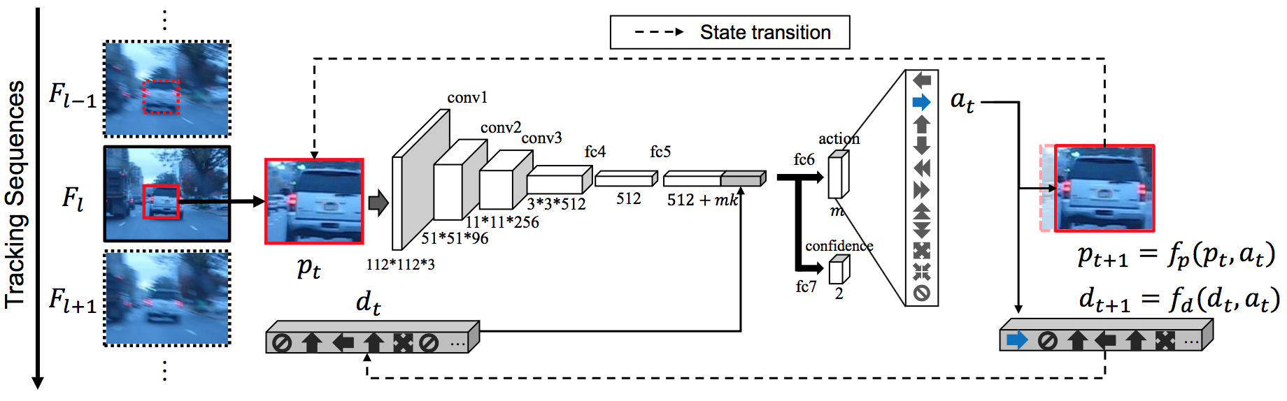
Action-Decision Network (ADNet): For each frame (\(F_l\)) in a video, a sequence of actions is predicted (in a markov decision process manner). Each action \(a_t\) is predicted using a convolutional neural network that takes two inputs: a patch \(p_t\) (i.e. target image slightly shifted or scaled) and an action dynamics vector \(d_t\) (a history of previously predicted actions). Once a "stop" action is predicted, ADNet accepts the last bounding box as the target's location and moves to the next frame \(F_{l+1}\) [25].
[25] presents a unique approach to solving the object tracking problem. Instead of regressing over the object location in each position, it would instead predict a sequence of actions. After applying these actions, the tracker obtains a new bounding box that indicates the object’s location in the new frame. Iteratively, the tracker repeats that process over consecutive frames through the test sequence. The actions are proposed by an Action-Decision Networks (ADNets). The ADNets are pretrained using supervised learning. Later, the network is trained in a reinforcement learning fashion to predict next action given current state. During tracking, online adaptation is applied to recaliberate the network.
Markov Decision Process
The authors presented a tracker that follows a Markov Decision Process with the following parameters:
where is the state at step , is the predicted action for that step, is the state at step resulting from applying action to state using the state transition function , and the reward for predicting the action for state .
The Markov process happens on two levels: frame and action levels. In other words, within a video, we only predict the bounding box in the next frame based only on the current frame. On the action level, we transition to the next state (and thus, the bounding box location) based only on the current state and action . The action is predicted based on current state .
Action
The action space is a discrete space with a total of 11 actions. Any action is represented as an 11-dimensional one-hot-encoded vector.
State
A state is defined as a tuple of a “patch” and an “action dynamics vector” .
The action dynamics vector is a flattened vector of the most recent 10 actions. The vector is 110-dimensional because each action is encoded as an 11-dimensional vector (thus, ).
The patch is a frame image that is obtained using the function . The function is a pre-processing function that cuts the a patch of an image according to the bounding box and resizes it to fit the network’s input (i.e. ).
The bounding box is defined by its center , width and height .
State Transition Function
The action transition function is responsible for applying the action to the state to transition to the next state .
The next state consists of boundary box, , and an action dynamics vector, .
The new decision boundary is obtained using the function . is the unit of change along the x-axis. is the unit of change along the y-axis. is a hyperparameter that [25] estimated experimentally to be .
In , the new action dynamics vector is obtained by concatenating the current action to the existing actions dynamic vector, . During concatenating, the oldest action () gets removed to make space for the most recent one (i.e. ).
When “Stop” action is received (at step, ), the agent will receive the reward for the current frame. The current state will be transferred to the next frame as the initial state where we repeat the previous process.
Reward
The reward function only depends on the final state () for each frame (i.e. the last state at the Markov Decision Process). We reward the network only on predictions whose Intersection-over-Union (IoU) is greater than . The reward is used for training the model in reinforcement learning (in the policy gradient method).
Action Classification
ADNet is a convolutional neural network used for predicting an action given the current state. Given the patch , the network predicts probabilities for each action (i.e. ). We choose the action, , that maximizes that probability.
Convolutional Layers
The authors used transfer learning in their solution as they initialized their network with a pre-trained VGG-M [30]. They choose a rather small model (instead of deep learning approaches) as it proves more effective in visual object tracking.
Their network consists of three convolutional layers, {conv1, conv2, conv3}. The convolutional layers are good feature extractors for the later action probability prediction and target/background confidence prediction layers. The feature maps are fed to two fully connected layers, {fc4, fc5}, both of which are combined with ReLU and Dropout layers. Each one yield in a 512 units. The fc5 layer’s output is concatenated with the action dynamics vector. That adds up an additional 110 units, increasing the total output to units.
Action Prediction
A fully connected layer is responsible for predicting the actions probabilities, where are the weights for the whole network. That layer is fed with the 622 units from previous layer and predicts probabilities for the 11 actions in our action space, .
Target Confidence
A confidence layer, fc7, is used to predict the probability of target in a given state. This confidence probability is used for online adaptation during tracking.
Dataset
To train ADNet, the authors used 360 videos from the following datasets: ALOV300 [31], VOT2013 [31], VOT2014 [32], VOT2015 [33]. For evaluation purposes, they used OTB-50 [34] and OTB-100 [35] datasets. They excluded overlapping videos among training and testing datasets.
Network Training
The ADNet is trained both online and offline. Offline training includes both supervised and reinforcement learning. In online training, an online adaptation process is applied.
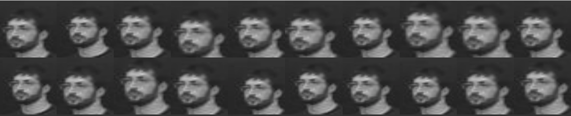 (a) Positive Samples | 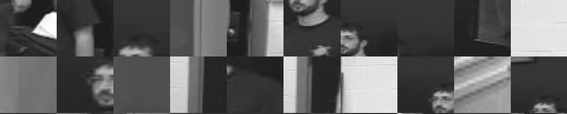 (b) Negative Samples |
Supervised Learning
The ADNet is trained on a randomly generated set of training samples. The training samples consist of image patches , action labels and class labels . The action dynamics vector is set to zero and is not used for training. At this phase, we train all network weights.
Sample Generation
The training videos provide video sequences along with per-frame (or, every k-th frame) bounding box annotations (). [25] applies gaussian noise to the bounding boxes and obtains .
As previously shown, the sampled bounding boxes are used to generate the patches . We could also infer the actions and class labels , as follows:
Loss Function
A multi-task loss function is used. The loss function is defined, as follows:
where and are the predicted action and class by ADNet, respectively.
Update Rule
The network was trained using stochastic gradient descent. The training makes 300 passes over each video. We draw 250 samples per frame from our gaussian noise distribution. Mini-batch size is 128. Learning rate is for convolutional layers and for fully connected layers. Momentum is and weight decay is .
| Tracking Simulation: During reinforcement learning, the network predicts bounding boxes for \(l\) frames (where \(l = 1 ... \mathcal{L}\)). For each frame, \(k\) actions are predicted (where \(k = 1 ... K_l\)). After \(\mathcal{L}\) frames, a reward is calculated and assigned to all previous actions. In other words, all actions leading to the resulting bounding box at frame \(\mathcal{L}\) will be equally rewarded or penalized [25]. |
Reinforcement Learning
In this phase, we train all network weights except the last layer.
Since the purpose of the reinforcement learning training is to learn the state-action policy, we ignore the confidence layer (fc7) during this phase. is initialized by the supervised learning wrights . Action dynamics vector is updated in every iteration to include the latest 10 actions and shifting them in first-in-first-out strategy.
Sample Generation
We randomly pick a training sequence with its ground truth data. After that, tracking simulation is used to generate a set of sequential states and their respective actions for the action steps and frames . Rewards are calculated at the last action step for each frame (i.e. at the -th step). The reward equation is used to calculate the reward. Note that all action states get the same reward (that of the last step, ).
Update Rule
Given states , actions and rewards , we use stochastic gradient ascent to maximize the scores as follows,
The reinforcement learning uses the same hyperparameters as those in the supervised learning.
It is worth noting that reinforcement learning introduces a form of semi-supervision. Usually, ground truths are not given for every frame but for every -th frame. The frames in between don’t have annotations. Thus, they could not be used in supervised learning. However, in reinforcement learning, we could use the reward of the -th frame for all non-annotated frames as they contribute to the current reward.
Online Adaptation
During tracking, ADNet updates its latent weights to learn more about the tracked object. This helps store information about the object’s shape from previous frames in the networks weights. That information helps the network recover from occlusions. In other words, the convolutional layers would contain video-agnostic generic information where the latent layers would contain video-specific information. The authors adopt the online adaptation proposed by [36].
Sample Generation & Finetuning
Similar to supervised learning, we need a training set of patches , action labels and class labels . In the first frame, a patch is given and its bounding box. We randomly sample bounding boxes from the original one. Then, we annotate their actions and classes, respectively. The initial training set is used to fine-tune the network for the first time.
After the first frame (), we update the network weights every frames. The training set samples bounding boxes over the past frame predictions whose confidence .
Re-detection
In cases where the confidence of the predicted bounding box is , we consider that the network missed its target and conduct a re-detection to capture the missing target.
The underlying assumption is that the missed target is in the vicinity of our prediction. Therefore, we pick our candidates by adding gaussian noise to our prediction. Finally, we choose the candidate that maximizes the class confidence.
Experimental Results
OTB-50 and OTB-100 datasets have been used for evaluating the ADNet’s performance, precision and success against other trackers (MDNet [24], C-COT [29], DeepSRDCF [15], HDT [37], MUSTer [13], MEEM [4], SCT [26], KCF [27], DSST [26] and GOTURN [12]). The experiments were conducted using an i7-4790K CPU, 32 GB RAM, and GTX TITAN X GPU, MATLAB2016b and MatConvNet toolbox [25].
The experimental results are obtained in a One-Pass Evaluation (OPE) manner while measuring precision and success on a frame-by-frame basis. One-pass evaluation means that trackers have been given the initial bounding box at the beginning of the video and bounding boxes are observed for all consecutive frames till the end of the video. The observed bounding boxes are then compared against the ground truth and success and precision are calculated. Success refers to the intersection-over-union (IoU). In the presented experiments, a “success” is defined by . Precision refers to the closeness of the predicted bounding box center coordinates to those of the ground truth. A “precise” prediction is achieved when the euclidean distance between predicted bounding box’s center and the ground truth’s center is less than 20 pixels.
The experimental results presented in [25] could be summarized as follows:
- Using reinforcement learning and supervised learning proves to achieve higher precision and success than just using supervised learning to train the action-decision network (i.e. action classifier).
- ADNet precision and success is comparable to the state-of-the-art (i.e. ~2.9% lower precision than MDNet and C-COT). However, it performs 3 times faster than both trackers.
- With change of hyperparameters (i.e. decreasing re-detection samples and online-adaptation samples), ADNet-fast achieves state-of-the-art precision and success among real-time trackers.
- Only 9% of all frames failed to detect track the target and used re-detection.
- Only 4% of all frames require more than 5 actions to localize the target in the next frame.
- The average number of searching steps (including actions predicted per frame and number of candidates in re-detection steps) is 28.26 step per frame. That compares favorably to the state-of-the-art tracker, MDNet, that requires 256 searching steps per frame.
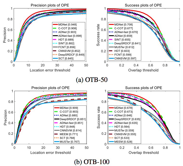 Success & Precision Plots: Top 10 trackers have been used to benchmark against ADNet and ADNet-fast on OTB-50 [34] and OTB-100 [35]. Namely, MDNet and C-COT achieve higher precision and success than ADNet and ADNet-fast [25]. |
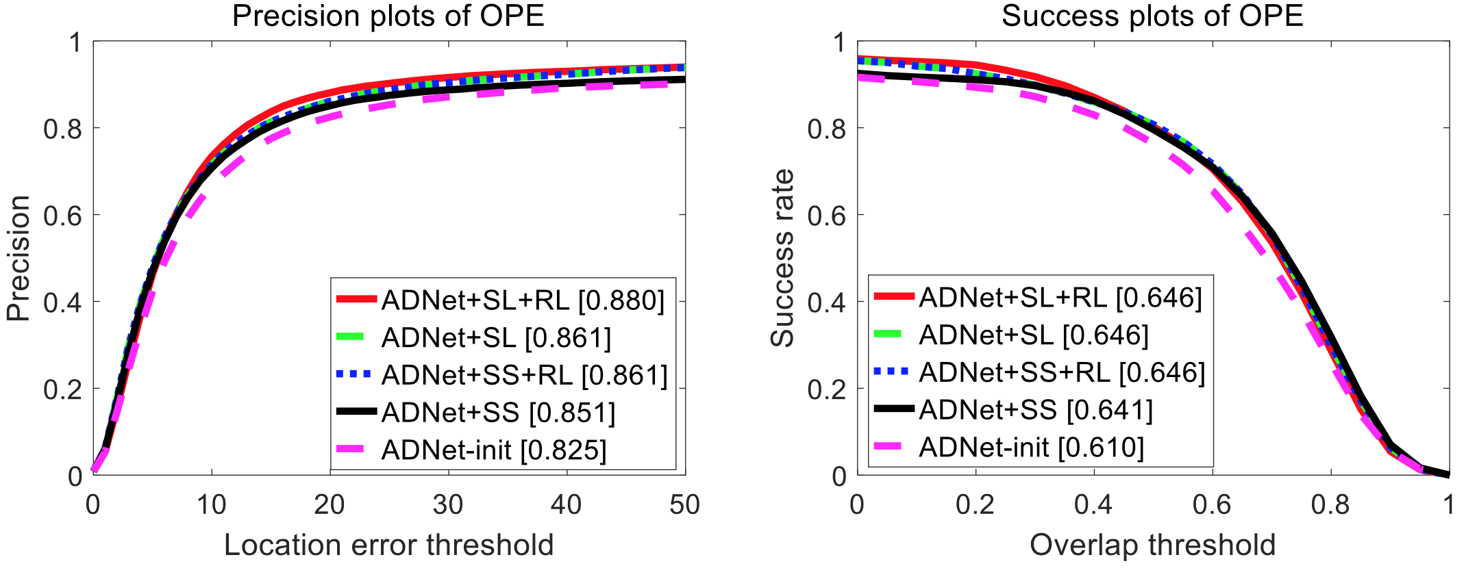
ADNet Component Analysis: Combining reinforcement learning with supervised learning (RL + SL) improves both mean precision and success over just using supervised learning (SL) [25].
Discussion
[25] poses a unique solution to the visual tracking problem. ADNet bypassed lots of problems faced by others (i.e. [12]): fault tolerance, search region parameterization, coordinate ranges parameterization, generalization to unseen targets, and semi-supervised learning for unlabelled frames. However, it also introduces some disadvantages: endless loops in markov decision process and an increased complexity.
Fault Tolerance
Early regression-based classifiers did not employ any confidence metric [12]. Thus, they could not predict if its regression is correct or wrong. That caused an error propagation throughout the frames sequence (i.e. causing more error in later frames). That problem was addressed by the ADNet architecture by employing a confidence classifier. The network uses the confidence prediction to detect potential failure and applies Re-detection to correct the missed targets.
Search Region
Regression-based networks need a lookup region where the target object is likely to be found. That introduced a new hyperparameter in some classifiers [12]. If the search region is too small, fast-moving objects would be entirely out of frame and won’t be localized. If the search region is too large, then the network slows down. ADNet avoids this entirely by infering actions (or, “moves”) given the bounding box in the next frame. If object is not found, then it zooms out and adapts to the fast-moving target objects.
Coordinate Ranges
Pixel-value regression poses many challenges to real-world applications. Different sequences have different resolutions. A network that is trained on low resolution images would predict lower pixel values and vice versa. Architectures tend to normalize pixel values into a specific domains (i.e. or ). That introduces another hyperparameter to tune. Small ranges cause the network to be insensitive to target object changes and vice versa. If the network is trained on low resolution images, it would make larger shifts in higher resolutions.
ADNet avoids this by predicting action applied to the target object. Moves and scales are relative to the target object size (rather than the frame size); thus, it is robust in higher and lower resolution environments.
Generic Targets
The recent deep learning architectures used offline training in order to learn a generic search function among two consecutive frames. That improves the tracking accuracy among traditional online tracking tools. However, it also comes with a prior of seen objects. If the network is previously trained on faces, it tends to track them better than other objects.
ADNet combines both offline training with online tracking to keep information about the target object. Instead of storing the target in a template database, it uses Online Adaptation to backpropagate the target information to its latent layers (fully connected layers for confidence and action prediction). That helps the network to generalize and track new objects.
Semi-supervised Learning
Existing datasets are not labeled frame-by-frame. Instead, they are labeled every 2nd, 3rd or even 5th frame. For example, ALOV300 [31] is labeled every 5th frame. That shrinks the size of the training data to 20% of the available frames. In supervised learning, networks use the labelled data. Some (i.e. [12]) introduce motion models that augment the labelled data by using still images (from ImageNet [38]).
ADNet mitigates this problem by using reinforcement learning on unlabelled frames. In tracking simulation, unlabelled frames contribute to the final bounding box. Therefore, predictions over unlabelled frames are either penalized or rewarded and contribute to the model’s knowledge.
Endless Loops
In markov decision process, an action is predicted iteratively till a “stop” action is observed. That raises the following question: “What if a stop action is never predicted?” Another problem is predicting actions that cancel each other. For example, a sequence of left, right and left moves, yields in the original object location. A more subtle example would be: left, left, top, down, right, right. Loops are unclear in these scenarios. The authors handle the simple loop cases (i.e. left-right-left scenarios). However, they don’t discuss or present any details if longer, more complex loops occur.
Network Complexity
ADNet requires many steps in training (pre-training using supervised learning, reinforcement learning, online adaptation). Its implementation is also quite difficult. Unlike simpler architectures like GOTURN [12], it requires many iterations to detect a target among two frames.
ADNet evaluated the impact of each learning method on their resulting architecture. However, they did not evaluate the markov decision process, online adaptation, re-detection or action dynamics vector contributions to their overall precision and success. Another pitfall was benchmarking against GOTURN who trained on ALOV300 and still images from ImageNet where their solution trained on ALOV300, VOT2013, VOT2014 and VOT2015. ADNet simply saw more data than GOTURN. Online adaptation biases the network to track a specific object. That improves accuracy. However, it also fails in scenarios with highly deformable targets (i.e. diving sequence in VOT2013).
In a future work, I would like to add online adaptation, confidence prediction and re-detection to a simpler architecture like GOTURN and measure their impact on its performance. That will also help better understand the improvement from action prediction rather than bounding box regression.
Conclusion
ADNet proposes a new architecture for visual object tracking. The proposed solution predicts a sequence of actions to be carried out to obtain the bounding box in the next frame. It uses supervised learning to pre-train the action-decision network that is later trained using reinformcement learning. Reinforcement learning enables a form of semi-supervised learning where the network learns from unlabeled frames. During testing, online adaptation is used to store object-specific information in the latent layers. That helps keep contextual information and results in better confidence prediction. In case of missing the target object, a re-detection is carried out to find the bounding box that maximizes the predicted confidence. A thinned out version of ADNet (ADNet-fast) outperforms state-of-the-art realtime trackers.
Live Demo
Presentation
Acknowledgements
- This article is not referring to a novel work of mine (“Yehya Abouelnaga”). Instead, it was conducted as a report for a class in which I implemented the ADNet network.
- “We” is often used in this article and refers to the authors of the ADNet paper.
- Most pictures are quoted from the authors of the ADNet paper (and are accordingly cited in this article).
References
- [1]Q. Wang, “Visual Tracker Benchmark Results,” GitHub. 2018 [Online]. Available at: https://github.com/foolwood/benchmark_results
- [2]M. Kristan et al., “A Novel Performance Evaluation Methodology for Single-Target Trackers,” IEEE Transactions on Pattern Analysis and Machine Intelligence, vol. 38, no. 11, pp. 2137–2155, Nov. 2016.
- [3]X. Li, W. Hu, C. Shen, Z. Zhang, A. Dick, and A. V. D. Hengel, “A Survey of Appearance Models in Visual Object Tracking,” ACM Trans. Intell. Syst. Technol., vol. 4, no. 4, p. 58:158:48, Oct. 2013 [Online]. Available at: http://doi.acm.org/10.1145/2508037.2508039
- [4]J. Zhang, S. Ma, and S. Sclaroff, “MEEM: robust tracking via multiple experts using entropy minimization,” in European Conference on Computer Vision, 2014, pp. 188–203.
- [5]S. Gu, Y. Zheng, and C. Tomasi, “Efficient visual object tracking with online nearest neighbor classifier,” in Asian Conference on Computer Vision, 2010, pp. 271–282.
- [6]Z. Han, J. Jiao, B. Zhang, Q. Ye, and J. Liu, “Visual object tracking via sample-based Adaptive Sparse Representation (AdaSR),” Pattern Recognition, vol. 44, no. 9, pp. 2170–2183, 2011 [Online]. Available at: http://www.sciencedirect.com/science/article/pii/S0031320311000872
- [7]Z. Yin, F. Porikli, and R. T. Collins, “Likelihood Map Fusion for Visual Object Tracking,” in 2008 IEEE Workshop on Applications of Computer Vision, 2008, pp. 1–7.
- [8]Z. H. Khan, I. Y. H. Gu, and A. G. Backhouse, “Robust Visual Object Tracking Using Multi-Mode Anisotropic Mean Shift and Particle Filters,” IEEE Transactions on Circuits and Systems for Video Technology, vol. 21, no. 1, pp. 74–87, Jan. 2011.
- [9]D. Comaniciu, V. Ramesh, and P. Meer, “Kernel-based object tracking,” IEEE Transactions on Pattern Analysis and Machine Intelligence, vol. 25, no. 5, pp. 564–577, May 2003.
- [10]D. S. Bolme, J. R. Beveridge, B. A. Draper, and Y. M. Lui, “Visual object tracking using adaptive correlation filters,” in 2010 IEEE Computer Society Conference on Computer Vision and Pattern Recognition, 2010, pp. 2544–2550.
- [11]N. Wang and D.-Y. Yeung, “Learning a deep compact image representation for visual tracking,” in Advances in neural information processing systems, 2013, pp. 809–817.
- [12]D. Held, S. Thrun, and S. Savarese, “Learning to track at 100 fps with deep regression networks,” in European Conference on Computer Vision, 2016, pp. 749–765.
- [13]Z. Hong, Z. Chen, C. Wang, X. Mei, D. Prokhorov, and D. Tao, “Multi-store tracker (muster): A cognitive psychology inspired approach to object tracking,” in Proceedings of the IEEE Conference on Computer Vision and Pattern Recognition, 2015, pp. 749–758.
- [14]Y. Qi et al., “Hedged deep tracking,” in Proceedings of the IEEE conference on computer vision and pattern recognition, 2016, pp. 4303–4311.
- [15]M. Danelljan, G. Hager, F. Shahbaz Khan, and M. Felsberg, “Convolutional features for correlation filter based visual tracking,” in Proceedings of the IEEE International Conference on Computer Vision Workshops, 2015, pp. 58–66.
- [16]M. Danelljan, A. Robinson, F. S. Khan, and M. Felsberg, “Beyond correlation filters: Learning continuous convolution operators for visual tracking,” in European Conference on Computer Vision, 2016, pp. 472–488.
- [17]X. Wang, C. Li, B. Luo, and J. Tang, “SINT++: Robust Visual Tracking via Adversarial Positive Instance Generation,” in Proceedings of the IEEE Conference on Computer Vision and Pattern Recognition, 2018, pp. 4864–4873.
- [18]A. He, C. Luo, X. Tian, and W. Zeng, “A twofold siamese network for real-time object tracking,” in Proceedings of the IEEE Conference on Computer Vision and Pattern Recognition, 2018, pp. 4834–4843.
- [19]J. Choi et al., “Context-aware Deep Feature Compression for High-speed Visual Tracking,” in Proceedings of the IEEE Conference on Computer Vision and Pattern Recognition, 2018, pp. 479–488.
- [20]B. Li, J. Yan, W. Wu, Z. Zhu, and X. Hu, “High Performance Visual Tracking With Siamese Region Proposal Network,” in Proceedings of the IEEE Conference on Computer Vision and Pattern Recognition, 2018, pp. 8971–8980.
- [21]C. Sun, D. Wang, H. Lu, and M.-H. Yang, “Learning spatial-Aware regressions for visual tracking,” in Proceedings of the IEEE Conference on Computer Vision and Pattern Recognition, 2018, pp. 8962–8970.
- [22]Y. Song et al., “VITAL: VIsual Tracking via Adversarial Learning,” arXiv preprint arXiv:1804.04273, 2018.
- [23]R. Tao, E. Gavves, and A. W. M. Smeulders, “Siamese instance search for tracking,” in Proceedings of the IEEE conference on computer vision and pattern recognition, 2016, pp. 1420–1429.
- [24]H. Nam and B. Han, “Learning multi-domain convolutional neural networks for visual tracking,” in Proceedings of the IEEE Conference on Computer Vision and Pattern Recognition, 2016, pp. 4293–4302.
- [25]S. Yun, J. Choi, Y. Yoo, K. Yun, and J. Y. Choi, “Action-Decision Networks for Visual Tracking with Deep Reinforcement Learning,” 2017 IEEE Conference on Computer Vision and Pattern Recognition (CVPR), pp. 1349–1358, 2017 [Online]. Available at: http://ieeexplore.ieee.org/document/8099631/
- [26]J. Choi, H. Jin Chang, J. Jeong, Y. Demiris, and J. Young Choi, “Visual tracking using attention-modulated disintegration and integration,” in Proceedings of the IEEE Conference on Computer Vision and Pattern Recognition, 2016, pp. 4321–4330.
- [27]M. Tang, B. Yu, F. Zhang, and J. Wang, “High-speed Tracking with Multi-kernel Correlation Filters,” in Proceedings of the IEEE Conference on Computer Vision and Pattern Recognition, 2018, pp. 4874–4883.
- [28]A. Krizhevsky, I. Sutskever, and G. E. Hinton, “Imagenet classification with deep convolutional neural networks,” in Advances in neural information processing systems, 2012, pp. 1097–1105.
- [29]M. Danelljan, A. Robinson, F. S. Khan, and M. Felsberg, “Beyond correlation filters: Learning continuous convolution operators for visual tracking,” Lecture Notes in Computer Science (including subseries Lecture Notes in Artificial Intelligence and Lecture Notes in Bioinformatics), vol. 9909 LNCS, pp. 472–488, 2016.
- [30]K. Chatfield, K. Simonyan, A. Vedaldi, and A. Zisserman, “Return of the Devil in the Details: Delving Deep into Convolutional Nets,” CoRR, vol. abs/1405.3, 2014 [Online]. Available at: http://arxiv.org/abs/1405.3531
- [31]A. W. M. Smeulders, D. M. Chu, R. Cucchiara, S. Calderara, A. Dehghan, and M. Shah, “Visual tracking: An experimental survey,” IEEE Transactions on Pattern Analysis & Machine Intelligence, no. 1, p. 1, 2013.
- [32]M. Kristan et al., “The Visual Object Tracking VOT2014 Challenge Results,” in Computer Vision - ECCV 2014 Workshops, Cham, 2015, pp. 191–217.
- [33]M. Kristan et al., “The visual object tracking vot2015 challenge results,” in Proceedings of the IEEE international conference on computer vision workshops, 2015, pp. 1–23.
- [34]Y. Wu, J. Lim, and M.-H. Yang, “Online object tracking: A benchmark,” in Proceedings of the IEEE conference on computer vision and pattern recognition, 2013, pp. 2411–2418.
- [35]Y. Wu, J. Lim, and M.-H. Yang, “Object tracking benchmark,” IEEE Transactions on Pattern Analysis and Machine Intelligence, vol. 37, no. 9, pp. 1834–1848, 2015.
- [36]H. Nam and B. Han, “Learning Multi-Domain Convolutional Neural Networks for Visual Tracking,” CoRR, vol. abs/1510.0, 2015 [Online]. Available at: http://arxiv.org/abs/1510.07945
- [37]Y. Qi et al., “Hedged Deep Tracking,” 2016 IEEE Conference on Computer Vision and Pattern Recognition (CVPR), pp. 4303–4311, 2016 [Online]. Available at: http://ieeexplore.ieee.org/document/7780835/
- [38]J. Deng, W. Dong, R. Socher, L.-J. Li, K. Li, and L. Fei-Fei, “Imagenet: A large-scale hierarchical image database,” in Computer Vision and Pattern Recognition, 2009. CVPR 2009. IEEE Conference on, 2009, pp. 248–255.