Multi-Instance Learning for Sentiment Analysis
Introduction
Sentiment Analysis is the tasks of identifying the sentiment in a given text. It usually have different granularity: sentence-level or document level. In this report, we are mostly interested in product reviews. Therefore, our document unit is the review as a whole. We don’t have any pre-defined sentiments for review sentences. Therefore, for some of our approaches we propagate the review sentiment to its sentences. In a multi-instance learning alternative, we focus only on the sentiment of the review. In this report, we propose different architectures that tackle the sentiment analysis problem using different granularity: the review, the sentence and a combination of both.
Background
Sentiment Analysis
Sentiment Analysis is a classification task where a classifier infers the sentiment in a given document. The sentiment could usually be: positive, negative or neutral. It could also follow the 5-star ratings/scores that are presented in the Amazon Reviews datasets. A third alternative would be to define the problem as a binary classification problem where sentiment is either positive or negative. Throughout this document, we assume that sentiment is a multi-class problem; Therefore, any review has to have a Positive (p), Negative (n) or Neutral (0) label. For mapping Amazon’s 5-star rating to our three-label sentiment, we use the following mapping function:
Transfer Learning
Transfer learning is the art of training a complex model on a relatively large dataset (to avoid overfitting) and fine-tuning the pre-trained model on a smaller dataset. For example, in image classification, a convolutional network could be pre-trained on a large dataset like ImageNet, and then re-used on another classification task with limited amount of data. In this project, we apply the same concept; We train on a large dataset (Amazon Fine Foods) and fine-tune on a smaller one (Organic Dataset).
Multi-Instance Learning
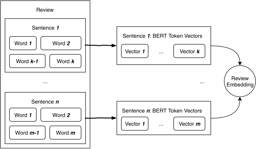
Inferring a review’s sentiment could take into account a multitude of dimensions. It could consider the review as a whole, as a bag of words (i.e. tokens) or as a bag of sentences.
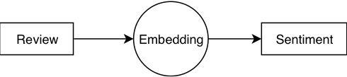
In single-instance learning, we consider a review as a whole; We extract features from the review regardless of its semantic structure. That usually leads to a fixed-width vector representation of any given review. In order to obtain that vector, we could use Xling, Bert [1], Word2vec [2], Glove [3], FastText [4] or fall back to TF-IDF embeddings. However, merging word-level or sentence-level embeddings into a review embedding makes a few assumptions: 1) that all words contribute equally to a sentence’s sentiment, and 2) that all sentences contribute equally to the review’s sentiment. Those assumptions are not necessarily true. Another downside is the negative correlation between review length (i.e. the number of tokens per review) and the contribution each token has on the overall sentiment.
 | 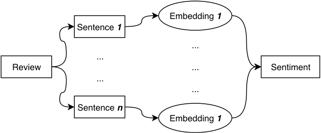 |
Multiple instance learning (MIL) is a variation of supervised learning where a single class label is assigned to a bag of instances. Multi-Instance learning avoids most of the pitfalls of the previous approach. Not all sentences affect sentiment equally. To account for that, we use smaller units (either tokens or sentences) to classify our sentiment. Finally, we reach a consensus by combining sentiment from the smaller units. We combine these result using majority voting (averaging all sentiments), weighted voting or using an attention-based mechanism.
In this report, we use both single- and multi-instance learning and compare the results.
Dataset
In this project, we worked with two main datasets: Amazon Fine Foods reviews and Organic Dataset. In this section, we would briefly describe both and mention problems we encountered with them.
 |  |
Amazon Fine Foods
Stanford SNAP’s uses a text file to store the reviews; Therefore, that makes it much faster to read partially (i.e. from the disk line by line). We created an adapter that reads that format and returns a generator. Our generator reads the following format:
...\
review/score: 3.0\
...\
review/text: The name and description of this Pickup \...
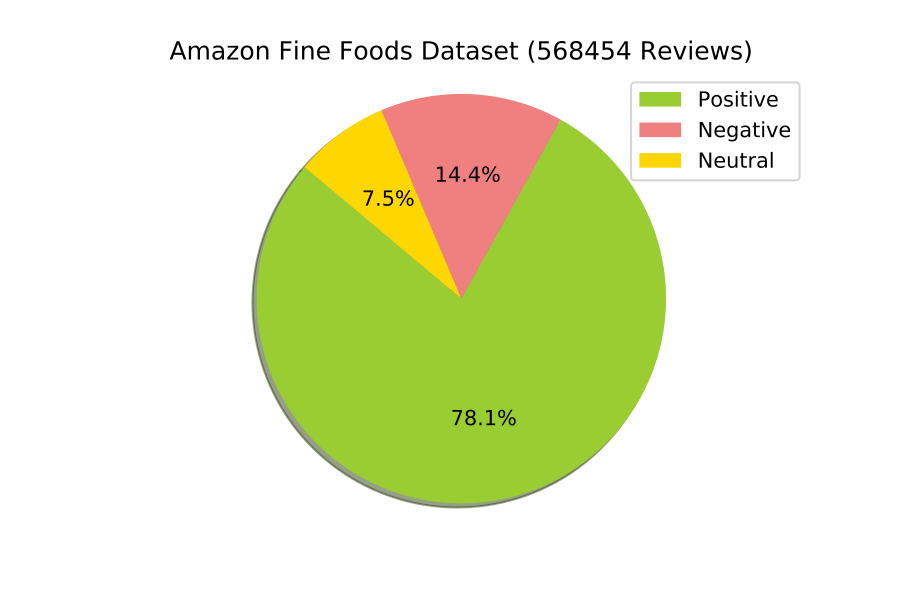
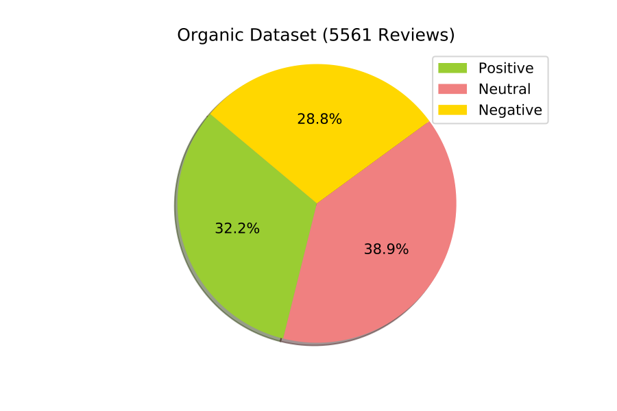
We encountered two main problems with the Amazon Fine Foods dataset. First is the class imbalance; As we could see in Figure [fig:label-distribution]{reference-type=”ref” reference=”fig:label-distribution”}, most of the fine foods reviews are positive. Therefore, we needed to use all reviews of the minority class and sample an equivalent number of reviews from the majority classes.
Second, we had a problem with fitting all reviews after converting them to BERT embeddings in memory. When pre-training most of the classifier, we trained and tested on 400,000 reviews (rather than the full 568,454 reviews). That accounted for 9 GB out of the 13 GBs available on Google Colab.
Organic Dataset
In order to use the Organic Dataset in our existing pipeline, we had to convert it to the SNAP text file format (see Figure [fig:stanford-snap-format]{reference-type=”ref” reference=”fig:stanford-snap-format”}). The snippet we used to do the conversion could be found in the appendix (see Appendix 7.3{reference-type=”ref” reference=”appendix:organic-to-snap-snippet”}).
The organic dataset comes with a new class of issues, mostly data quality related. In figure [fig:label-distribution]{reference-type=”ref” reference=”fig:label-distribution”}, we see that classes are fairly balanced. The dataset size is also very small therefore, we had no memory issues. However, when closely examining the data we find exact reviews that have different labels. For example, the following review exists twice and is labeled as both positive and negative: “For example, recently it came out that hen’s in certain types of ‘free range’ environments are actually worse off than battery hens.” Other reviews are lacking context, like “Improve their knowledge of farming and food production methods.”– which is labeled as neutral. To see more reviews with quality issues, you could have a look at the Appendix 7.4{reference-type=”ref” reference=”appendix:organic-quality-issues”}.
Experimental Setup
 {width=”.5\linewidth”} [[fig:colab-workflow]]{#fig:colab-workflow label=”fig:colab-workflow”}
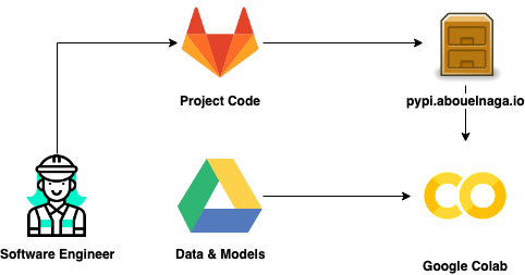
Google Colab Workflow
Google Colab is a fine tool to use for quick experimentation; However, in this practical course, it was the main driver to our experiments. That raised multiple challenges: data and model storage, version control, and timeouts (due to lengthy runtime). Model and storage was easy to solve by mounting our Google Drive to the notebooks we were working on. Sharing the models and data among team participants was as easy as reading/writing from/to a shared folder. Version control was trickier; We tried multiple attempts to attach this problem. One approach was to clone our git repositories in each session and then commit our changes as we go. That was inconvenient due to the lack of a text editor. Therefore, we decided to create our own packaging server and use it directly from Colab. To learn more about hosting our package server, refer to the Appendix 7.1{reference-type=”ref” reference=”section:hosting-pypi”}. For more information about what functionality our package contains, refer to Appendix 7.2{reference-type=”ref” reference=”section:tum-package”} or pypi.abouelnaga.io/tum.
Baselines: Logistic Regression, XGBoost & Bayesian Classifiers
{width=”.75\linewidth”} [[fig:baseline-features]]{#fig:baseline-features label=”fig:baseline-features”}
As a baseline in our experiments, we used the Scikit-Learn implementations of Logistic Regression Classifier, XGBoost Classifier and Gaussian Naive Bayes Classifier [5]. During training, we are feeding a single feature vector (the resulting embedding vector illustrated in Figure [fig:baseline-features]{reference-type=”ref” reference=”fig:baseline-features”}) of size 768 per review. Before the training step, we divide the whole database into 75%-25% splits. Validation sets come from 75% training split. On all classifiers, when pre-training on Amazon Fine Foods, we use only 400 chunks out of 569 chunks. Each chunk has a 1000 reviews. When fine-tuning on the Organic Dataset, we use the whole dataset (as it is relatively small).
Deep Feed Forward Network
- Layer Input Dense Dropout Dense Dropout Dense (Softmax)
- ————– ——- ——- ——— ——- ——— —————–
- Output Shape 768 128 128 64 64 3
-
Model Architecture for Deep Forward Network
[[table:feed-forward]]{#table:feed-forward label=”table:feed-forward”}
Our feed forward neural network is a simple extension to the baseline classifiers. In this step, we used Keras [6] on top of Tensorflow [7] to construct and train our model. Our model architecture is fairly simple (2 fully connected layers and 2 dropout layers; See Table [table:feed-forward]{reference-type=”ref” reference=”table:feed-forward”}). During both training and fine-tuning, we used an Adam optimizer and a categorical cross entropy loss. This model outperformed all other models on the Amazon Fine Foods dataset (see Table [table:results]{reference-type=”ref” reference=”table:results”}). However, when fine-tuning on the Organic Dataset, it did easily overfit. Overfitting happened from the first iteration and kept getting worse for this model (see Figure [fig:feed-forward-overfitting]{reference-type=”ref” reference=”fig:feed-forward-overfitting”} in Appendix 7.6{reference-type=”ref” reference=”appendix:feed-forward-overfitting”}).
Long Short Term Memory (LSTM)
 {width=”\linewidth”} [[fig:lstm]]{#fig:lstm label=”fig:lstm”}
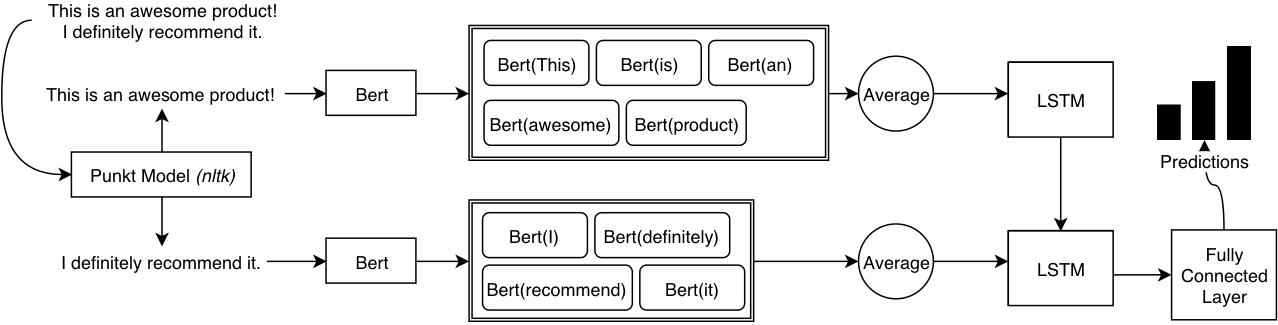
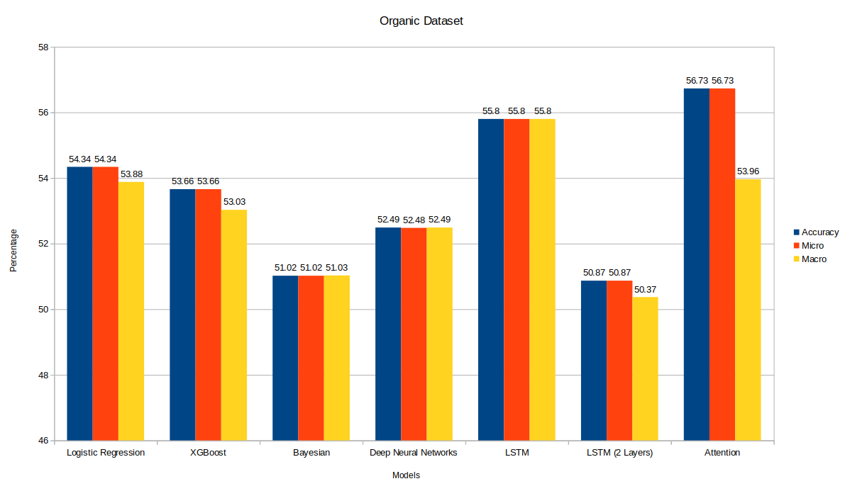
The baselines (Section 4.2{reference-type=”ref” reference=”section:baselines”}) and the Deep Feed Forward Model (Section 4.3{reference-type=”ref” reference=”section:feed-forward”}) produce decent results. However, they give equal weighting to each sentence in the review. That might work in a dataset where reviews tend to have many sentences (i.e. Amazon Fine Foods dataset). However, in the Organic Dataset, most reviews consist of one or two sentences. A model that learns features on a sentence-level is therefore a better fit for such a dataset. Therefore, we started to experiment with LSTMs on a sentence level. LSTMs performed worse (than the feed forward model) on the Amazon Fine Foods dataset and better on the organic dataset. That could be attributed to its using more LSTM steps in the Amazon reviews dataset which requires significantly more data to learn a better hidden state. The best performing LSTM model had only one layer LSTM with 25 hidden units. We experimented with using a two-layer LSTM model. That yielded the same performance on Amazon Fine Foods; However, its performance deteriorated significantly (i.e. 5% worse) on the Organic dataset.
Convolutional Net with Attention Mechanism
 {width=”\linewidth”} [[fig:architecture]]{#fig:architecture label=”fig:architecture”}
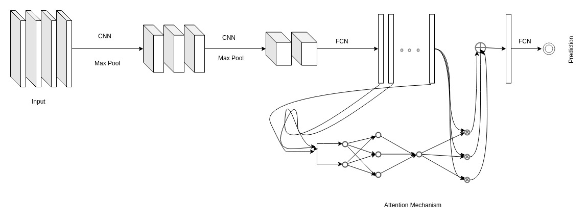
In this section, we adopt a Multi-Instance Learning (MIL) approach. MIL deals with problems where labels are associated with groups of instances or bags (reviews in our case), while instance labels (sentence-level sentiments) are unobserved. In this model, we use an attention mechanism [8] to learn an instance’s impact on the document’s label. More specifically, we use a convolutional network on words (per sentence) and then an attention mechanism to weigh sentences per review. We train the network end-to-end on review sentiment labels; Learned attention scores describe the weight a sentence has over the review’s sentiment. Attention scores use softmax (i.e. they sum up to 1). We are using the attention mechanism proposed in [9]. The authors propose that 1) all attention scores should sum up to one (i.e. using softmax), and 2) attention scores are to be applied to low-dimensional embedding vectors.
Preprocessing
We trained our model on Amazon Fine Food dataset and then fine-tuned on our Organic Dataset. We considered each review as our document and each sentence inside our review as instances. Data pre-processing involved similar steps as we did for our LSTM model (see Figure [fig:lstm]{reference-type=”ref” reference=”fig:lstm”}). Each review then became a bag of instances (sentences) having the shape of the number of sentences in the review where each sentence is represented by a feature vector of size 768. The bag level labels correspond to the labels of the reviews.
Training
The whole architecture can be seen as divided into four components.
-
The first component includes 1D convolution layers with ReLU activation and max pooling. The input (of size $R \times N \times 768$) is feed into a 1D convolution layer with ReLU activation. After that the feature maps go through a max-pooling layer, then again it goes through 1D convolution layer with ReLU activation and the feature maps are max pooled again; Thus, resulting in a feature vector of size $R \times N \times 25$.
-
The outputs of the previous component are fed into the second component, which composes Linear layers with ReLU activation and outputs feature vectors of size $R \times N \times 500$.
-
Outputs from the second component are then fed into the third component which is the Attention component. Attention component involves the layers accomplishing the attention mechanism. This component assigns weights to each instance of the bag (thus, yielding a weight vector of size, $R \times N \times 1$; One weight for each sentence). Attention scores (weights assigned to each instance) provides insight into the contribution of each instance to the bag label.
-
Finally, the outputs from the second ($\in R^{N \times 500}$) and third components ($\in R^{N \times 1}$) are multiplied (such that, $R^{1 \times N} \cdot R^{N \times 500} \longrightarrow R^{1 \times 500}$) and are fed to the fourth component, the classification component which is responsible for classifying a bag among Positive, Neutral or Negative (and thus, yields in $R \times 3$).
Results
We tried out several different combinations of network architectures (see Table [table:attention-best]{reference-type=”ref” reference=”table:attention-best”}, [table:attention-second-best]{reference-type=”ref” reference=”table:attention-second-best”} & [table:attention-third-best]{reference-type=”ref” reference=”table:attention-third-best”} in Appendix 7.8{reference-type=”ref” reference=”appendix:attention-different-architectures”}). We tried out different number of filters and kernel sizes for our convolutional component. We also replaced the convolutional component with FCN component in a few experiments but the results were better for convolutional component. We have shown here the results for some of our best network architectures (see Table [table:attention-results]{reference-type=”ref” reference=”table:attention-results”}). Training parameters are also presented in Table [table:optimizers]{reference-type=”ref” reference=”table:optimizers”}. An analysis of our attention scores per sentence is presented at Table [table:attention-scores]{reference-type=”ref” reference=”table:attention-scores”}.
Fine Tuning
The annotated Organic Dataset is preprocessed in a way that we have for each sentence a sentiment. Thus our bags of reviews have one sentence inside it, or in other words, each bag has a single instance inside it. We fed these bags to our models in the exact similar way as we did for the Amazon fine food bags. Fine-tuning was done using almost the same hyper-parameters except that the learning rate was reduced drastically and we fine-tuned it for longer epochs. The results are presented in the Attention Results table [table:attention-results]{reference-type=”ref” reference=”table:attention-results”}.
Results
Our results (see Table [table:results]{reference-type=”ref” reference=”table:results”}) have been very interesting. First, a parity between simple models like Linear Regression and LSTM and Deep networks was clear in our experiments; Simple models (i.e. Logistic Regression) seemed to perform as good (and sometimes even better) as our complex models (i.e. XGBoost and 2-Layered LSTM). Probabilistic estimation methods like bayesian classifiers were clearly lagging behind; But this is understandable given the high dimensionality of the problem. Organic dataset was very easy to overfit; Almost all of our best performing models (except 1-Layer LSTM) seemed to overfit after the first iteration. Majority voting (i.e. simple averaging) over review sentence BERT embeddings seemed to be very powerful (as demonstrated in our Logistic Regression, XGBoost, Bayesian Classifier, and Deep Feed Forward network).
Conclusion
In this report, we explore different architectures for the sentiment analysis problem. We were also interested in the applicability of transfer learning on a much smaller dataset (Organic Dataset). We approached the problem from two different perspectives: Single Instance Learning and Multiple Instance Learning. In Single Instance Learning, we unified all words in a review in one embedding (i.e. instance). Whereas for Multiple Instance Learning, we have a ground truth label for a batch of instances (sentences).
We started our experiments with baselines. We evaluated the performances of various baselines such as Logistic Regression, XGBoost Classifier, Bayesian Classifier, Deep Feed Forward Network. Then we went on to build our own architecture on top of BERT embeddings for sentences for the task of sentiment analysis. We tried Feed Forward networks with 2 fully connected layers and two Dropouts. We also tried two variants of LSTM. Then finally we moved towards implementing a CNN with an attention mechanism for multiple instance learning.
Throughout our work, we faced a variety of technical challenges due to using Google Colab resources for our research. These problems range from memory issues to simple timeout problems. We outlined our solution to all of these problems in detail throughout this report.
We’ve shown than simple models like Logistic Regression are powerful contenders for sentiment analysis. They don’t outperform the more advanced LSTM or attention-based models; However, the performance gap is not that high. An extension to this project would be to verify the above statement by training the same models that we presented here on different categories of the amazon reviews dataset. Another interesting extension would be to explore the relation a review’s length has on performance in different architectures.
References
- [1]J. Devlin, M.-W. Chang, K. Lee, and K. Toutanova, “Bert: Pre-training of deep bidirectional transformers for language understanding,” arXiv preprint arXiv:1810.04805, 2018.
- [2]T. Mikolov, K. Chen, G. Corrado, and J. Dean, “Efficient estimation of word representations in vector space,” arXiv preprint arXiv:1301.3781, 2013.
- [3]J. Pennington, R. Socher, and C. Manning, “Glove: Global vectors for word representation,” in Proceedings of the 2014 conference on empirical methods in natural language processing (EMNLP), 2014, pp. 1532–1543.
- [4]P. Bojanowski, E. Grave, A. Joulin, and T. Mikolov, “Enriching word vectors with subword information,” Transactions of the Association for Computational Linguistics, vol. 5, pp. 135–146, 2017.
- [5]F. Pedregosa et al., “Scikit-learn: Machine Learning in Python,” Journal of Machine Learning Research, vol. 12, pp. 2825–2830, 2011.
- [6]F. Chollet and others, “Keras.” \urlhttps://keras.io, 2015.
- [7]Martı́n Abadi et al., “ TensorFlow: Large-Scale Machine Learning on Heterogeneous Systems.” 2015 [Online]. Available at: https://www.tensorflow.org/
- [8]D. Bahdanau, K. Cho, and Y. Bengio, “Neural machine translation by jointly learning to align and translate,” arXiv preprint arXiv:1409.0473, 2014.
- [9]M. Ilse, J. M. Tomczak, and M. Welling, “Attention-based Deep Multiple Instance Learning,” arXiv preprint arXiv:1802.04712, 2018.
Appendix
Hosting our packaging server
There are two options to host a python packaging server: on the cloud, and on bare metal servers. On the cloud, we used Amazon Web Services S3 as a static website host. Now, deploying a package to the cloud was as easy as copying files from our local machines to the S3 Bucket. Here are more documentation on the process:
Finally, you could have a look at the package code on our server here: pypi.abouelnaga.io/tum.
The “tum” Package
As we created our own webserver, we wanted to have a portable version of our code. So we decided to create a package out of our most used functionality. The package contains helper functions to read from Amazon Reviews Dataset text file format (the one found on Stanford SNAP’s servers). It also contains more code that reads the reviews, divides them into sentences using NTLK, computes one-hot encoded labels, and runs BERT against the pre-computed sentences. During the course, we needed to pre-compute everything to speed our development. When we tried to pre-compute BERT embeddings, we bagan to face problems with memory sizes and disk writes.
On average, a 1000 reviews of the Amazon Fine Foods dataaset took 2̃5MB (after being converted to BERT vectors). Note that, here we are not storing all word embeddings; Instead, we are averaging all words per sentence. Therefore, the 25MB per 1000 reviews only correlates to the number of sentences per review. Therefore, if we have reviews with more sentences, then we store more BERT vectors (and thus consume more memory space).
To learn more about the package, you could see our documentation at: docs.abouelnaga.io/tum.
Transform Organic Dataset Into Amazon SNAP Text Format
``` {.python language=”Python”} import pandas as pd
def select_reviews_with_sentiment(df: pd.DataFrame): return df[df.Sentiment.notna()]
def convert_df_to_text(df, name=””): reviews = [] to_score = {“0”: 3.0, “p”: 5.0, “n”: 1.0} for i in range(df.shape[0]): score = to_score[df.iloc[i].Sentiment] sentence = df.iloc[i].Sentence reviews.append( f”review/score: {score}\n” f”review/summary: None\n” f”review/text: {sentence}\n” )
with open(f"{name}.txt", "wt") as f:
    f.write("\n".join(reviews))
GS = “/content/gdrive/My Drive/Colab Notebooks” organic_prefix = f”{GS}/organic-dataset/train_test_validation V0.2” organic_train_csv = f”{organic_prefix}/train/dataframe.csv” organic_val_csv = f”{organic_prefix}/validation/dataframe.csv” organic_test_csv = f”{organic_prefix}/test/dataframe.csv”
| df_train = pd.read_csv(organic_train_csv, delimiter=” | ”) |
| df_validate = pd.read_csv(organic_val_csv, delimiter=” | ”) |
| df_test = pd.read_csv(organic_test_csv, delimiter=” | ”) |
df_train = select_reviews_with_sentiment(df_train) df_validate = select_reviews_with_sentiment(df_validate) df_test = select_reviews_with_sentiment(df_test)
df_all_test = pd.concat([df_validate, df_test])
convert_df_to_text(df_train, name=f”{GS}/OrganicDataset.Train”) convert_df_to_text(df_all_test, name=f”{GS}/OrganicDataset.Test”)
Organic Dataset Reviews with Quality Issues {#appendix:organic-quality-issues}
-------------------------------------------

### Contradicting Labels

-   (Exists twice with positive & negative labels) For example, recently
    it came out that hen's in certain types of 'free range' environments
    are actually worse off than battery hens.

-   (Exists twice with positive & negative labels) You're not
    deliberately putting toxins in their mouths that their body should
    not be exposed to for optimal health.

-   (Exists thrice; Twice positive and once negative) So, this is more
    of a question regarding whether or not you personally think it's
    worth it not to consume toxins and support better agriculture
    methods.

-   (Exists twice; Positive and neutral) As someone who grew up on a
    farm I find people's awareness of modern farming methods to be
    abysmal.

### Lacking Context

-   Every purchase is a vote for what should be on the market.

-   'Organic' agriculture goes along with that theme, but certified
    organic is an over-reaction.

-   When it warms up we'll average about 7 a day.

-   That's more eggs then we can eat as a family of four.

-   The FDA was formed to fight dangerous food, drugs, and cosmetics,
    and is not beholden to agribusiness.

-   The EPA for formed to protect the environment, and is not beholden
    to agribusiness.

-   Organic farmers can legally use pesticides and many do.

Pre-computing labels, sentences and BERT Embeddings
---------------------------------------------------

Over the course of this work, we trained a variety of approaches to
train our classifiers. We tried use generators that will lazy load our
reviews, compute BERT embeddings and pass them to the classifier. That
proved very slow and with low benefit as we were not doing any kind of
data augmentation in the process. An alternative was to pre-compute and
cache everything ahead of time. That worked quite well for us and helped
us speed our experimentation dramatically. Our pre-computation logic
also lives in the "tum" package (see Appendix
[7.2](#section:tum-package){reference-type="ref"
reference="section:tum-package"}) and is exposed over its [Command Line
Interface (CLI)](http://docs.abouelnaga.io/tum/cli.html).

After installing the "tum" package, you could run the following snippet
in "bash" or "zsh":

``` {.bash language="Bash"}
tum download-amazon-reviews -c Arts 	# Downloads Arts.txt (from snap.stanford.edu)
tum precompute-labels -c Arts 		# Creates Arts.labels.npy
tum precompute-sentences -c Arts 	# Creates Arts.sentences.npy
tum precompute-bert -c Arts		# Creates Arts.bert.{chunk_id}.{chunk_size}.py
Deep Feed Forward Model Overfitting on Organic Dataset
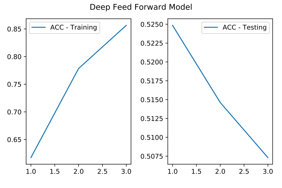 {width=”.75\linewidth”} [[fig:feed-forward-overfitting]]{#fig:feed-forward-overfitting label=”fig:feed-forward-overfitting”}
Experimental Results: Attention-based Mechanism
  Model      Accuracy   F1\_Macro   F1\_Micro
  Best        73.08       73.35       73.08    Second Best    74.26       74.17       74.26    Third Best     72.03       71.45       72.03   ------------- ---------- ----------- -----------
: Convolutional Network with Attention Results
  Model      Accuracy   F1\_Macro   F1\_Micro
  Best        56.73       53.96       56.73    Second Best      55        53.16        55   ------------- ---------- ----------- -----------
: Convolutional Network with Attention Results
[[table:attention-results]]{#table:attention-results label=”table:attention-results”}
Different Architectures with Attention
In this section we dive deeper into the details and experimentation with attention mechanism.
- Layer Type
- 1 Conv1d(768, 20, kernel_size=(1,), stride=(1,))
- 2 ReLU()
- 3 MaxPool2d(kernel_size=2, stride=2, padding=0, dilation=1, ceil_mode=False)
- 4 Conv1d(10, 50, kernel_size=(1,), stride=(1,))
- 5 ReLU()
- 6 MaxPool2d(kernel_size=2, stride=2, padding=0, dilation=1, ceil_mode=False)
- ——- ——————————————————————————
-
Attention-based Architecture: Best Performing Model
- Layer Type
- 1 Linear(in_features=25, out_features=500, bias=True)
- 2 ReLU()
- ——- ——————————————————-
-
Attention-based Architecture: Best Performing Model
- Layer Type
- 1 Linear(in_features=500, out_features=128, bias=True)
- 2 Tanh()
- 3 Linear(in_features=128, out_features=1, bias=True)
- ——- ——————————————————–
-
Attention-based Architecture: Best Performing Model
- Layer Type
- 1 Linear(in_features=500, out_features=3, bias=True)
- 2 Softmax()
- ——- ——————————————————
-
Attention-based Architecture: Best Performing Model
[[table:attention-best]]{#table:attention-best label=”table:attention-best”}
- Layer Type
- 1 Conv1d(768, 20, kernel_size=(1,), stride=(1,))
- 2 ReLU()
- 3 MaxPool1d(kernel_size=2, stride=2, padding=0, dilation=1, ceil_mode=False)
- 4 Conv1d(20, 50, kernel_size=(1,), stride=(1,))
- 5 ReLU()
- 6 MaxPool1d(kernel_size=2, stride=2, padding=0, dilation=1, ceil_mode=False)
- ——- ——————————————————————————
-
Attention-based Architecture: Second Best Performing Model
- Layer Type
- 1 Linear(in_features=50, out_features=500, bias=True)
- 2 ReLU()
- ——- ——————————————————-
-
Attention-based Architecture: Second Best Performing Model
- Layer Type
- 1 Linear(in_features=500, out_features=128, bias=True)
- 2 Tanh()
- 3 Linear(in_features=128, out_features=1, bias=True)
- ——- ——————————————————–
-
Attention-based Architecture: Second Best Performing Model
- Layer Type
- 1 Linear(in_features=500, out_features=3, bias=True)
- 2 Softmax()
- ——- ——————————————————
-
Attention-based Architecture: Second Best Performing Model
[[table:attention-second-best]]{#table:attention-second-best label=”table:attention-second-best”}
- Layer Type
- 1 Conv1d(768, 512, kernel_size=(1,), stride=(1,))
- 2 ReLU()
- 3 MaxPool2d(kernel_size=2, stride=2, padding=0, dilation=1, ceil_mode=False)
- 4 Conv1d(256, 256, kernel_size=(1,), stride=(1,))
- 5 ReLU()
- 6 MaxPool2d(kernel_size=2, stride=2, padding=0, dilation=1, ceil_mode=False)
- ——- ——————————————————————————
-
Attention-based Architecture: Third Best Performing Model
- Layer Type
- 1 Linear(in_features=128, out_features=500, bias=True)
- 2 ReLU()
- ——- ——————————————————–
-
Attention-based Architecture: Third Best Performing Model
- Layer Type
- 1 Linear(in_features=500, out_features=128, bias=True)
- 2 Tanh()
- 3 Linear(in_features=128, out_features=1, bias=True)
- ——- ——————————————————–
-
Attention-based Architecture: Third Best Performing Model
- Layer Type
- 1 Linear(in_features=500, out_features=3, bias=True)
- 2 Softmax()
- ——- ——————————————————
-
Attention-based Architecture: Third Best Performing Model
[[table:attention-third-best]]{#table:attention-third-best label=”table:attention-third-best”}
Experimental Results Plots
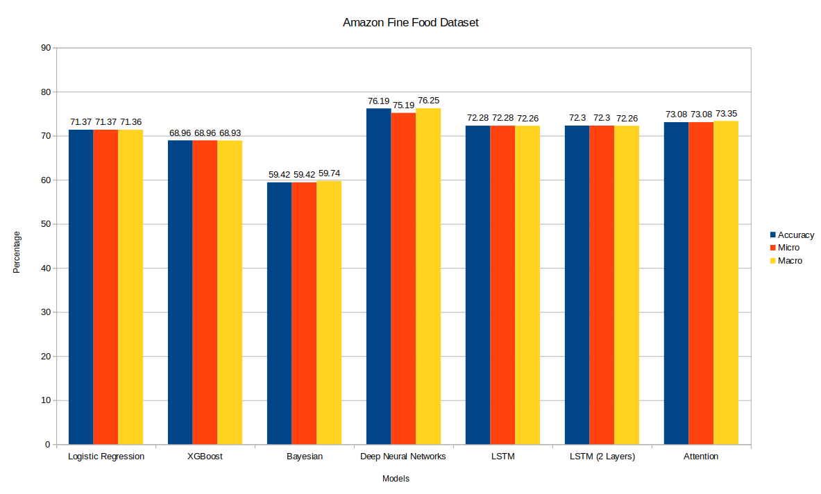 {width=”\linewidth”} [[fig:Results]]{#fig:Results label=”fig:Results”}
 {width=”\linewidth”} [[fig:Results]]{#fig:Results label=”fig:Results”}
- Review Attention Scores Target Label Predicted Label
- ——– ——————————– ————– —————–
- [[0.3479, 0.6521]] Negative Negative
- [[0.3723, 0.6277] Positive Positive
- [[0.4251, 0.4119, 0.1630]] Neutral Neutral
- [[0.3924, 0.6076]] Neutral Neutral
- [[0.1605, 0.1160, 0.7235]] Positive Positive
-
Review and Attention Scores.
[[table:attention-scores]]{#table:attention-scores label=”table:attention-scores”}
   Experiment       Optimizer                Learning Rate   Weight decay   Epochs     -------------------- ----------- ------------ --------------- -------------- -------- --    Fine Foods Dataset     Adam      0.9, 0.999      0.0005          0.0001      20-50
Organic Dataset       Adam      0.9, 0.999      0.00005         0.0001        50
: Training details for Convolutional Nets with Attention
[[table:optimizers]]{#table:optimizers label=”table:optimizers”}