Realtime Neural Object Recognition and 3D Pose Estimation

22 March 2018

Yehya Abouelnaga
Technical University of Munich

Introduction

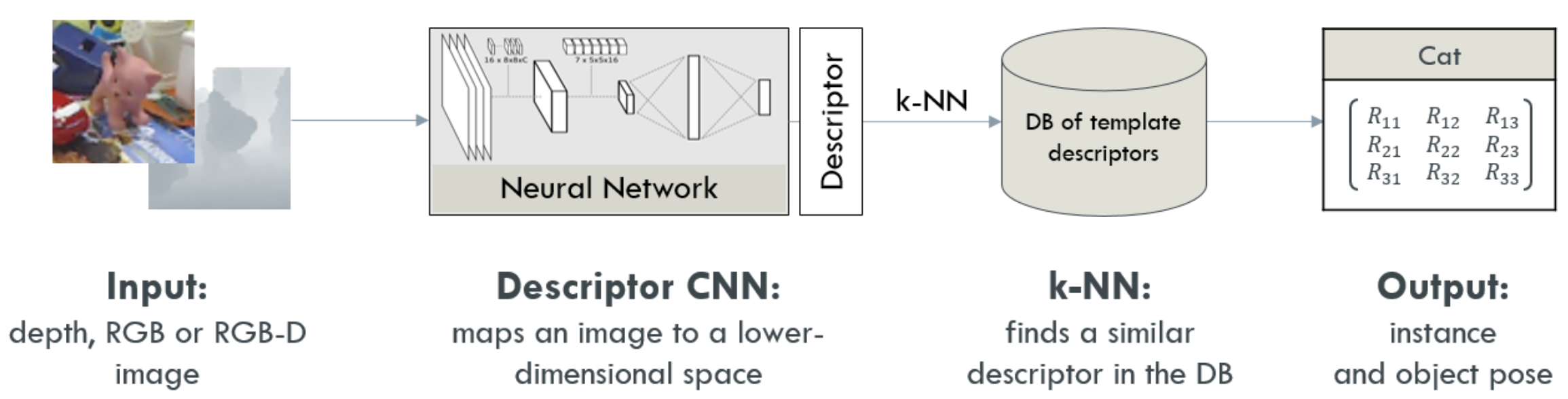
Object Recongition and 3D Pose Estimation are heavily researched topics in Computer Vision. They are often needed in emerging Robotics and Augmented Reality applications. Most common pose estimation methods use single classifier per object, and thus, resulting in a linear growth of complexity with every new object in the environment. In this project, I use a custom hinge-based loss to learn descriptor that separate objects based on their class and 3D pose. Learned feature space will be used in combination with k-nearest neighbour to detect object class and estimate its pose.

Note that this is a graduate class project conducted in the ‘‘Tracking and Detection in Computer Vision’’ class in the Technical University of Munich (TUM) taught by Dr. Slobodan Ilic. You could have a look at the Github repository.

Realtime Object Detection and 3D Pose Estimation Pipeline

Loss Function

Loss functions are key components in neural networks research. They guide the networks to approach a local minima that achieves a certain objective (i.e. classification or regression). In this project, I implement a custom hinge loss [1] that trains on triplets of anchors, pullers and pushers. The custom loss teaches the network to pull the "Pullers" close to the "Anchors" and to push the "Pushers" away from the "Anchors".

$L = L_{triplets} + L_{pairs}$ $L_{triplets} = \sum_{(s_a, s_+, s_-) \in T} \max \left( 0, 1 - \frac{ \left|\left| \, f(x_a) - f(x_-) \, \right|\right|_2^2 }{ \left|\left| \, f(x_a) - f(x_+) \, \right|\right|_2^2 + m } \right)$ $L_{pairs} = \sum_{(s_a, s_+) \in P} \left|\left| \, f(x_a) - f(x_+) \, \right|\right|_2^2$

Network Architecture

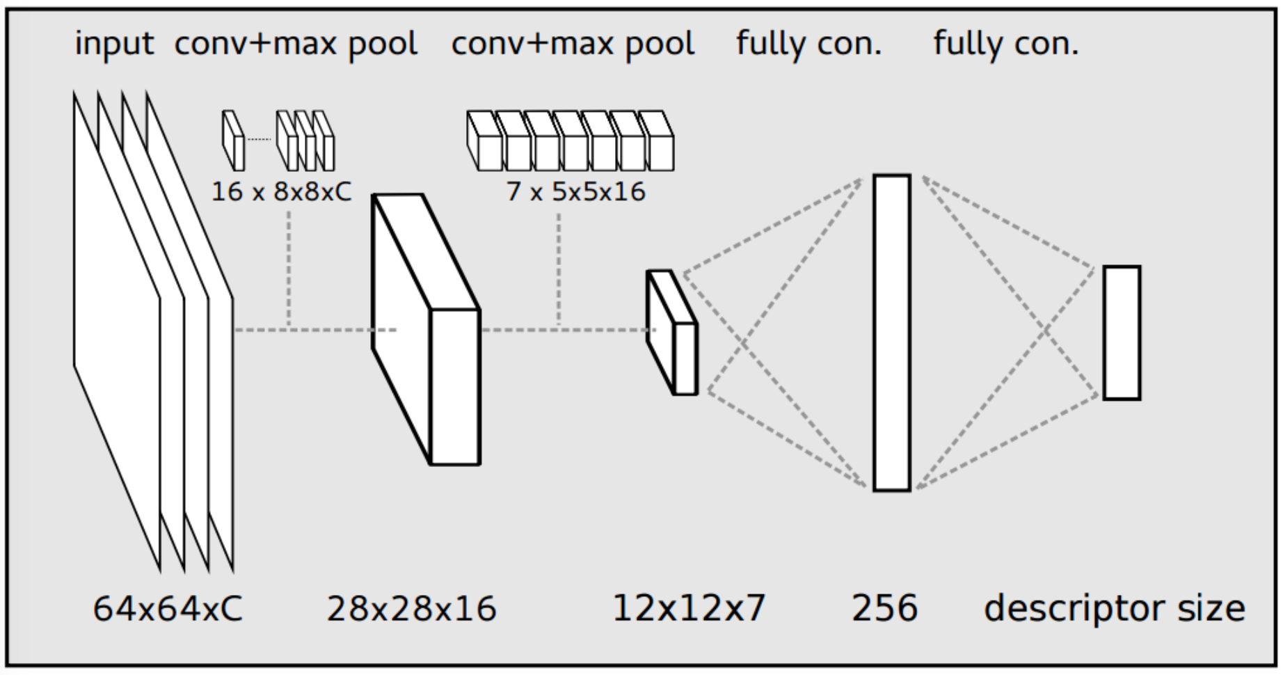Descriptor Architecture

Instead of verbosely describing the network architecture, you could find implemented below:

# num_classes = 5
input_dim = 64
channels = 3
hidden_size = 256
descriptor_size = 16

graph = {}

graph['learning_rate'] = tf.placeholder(tf.float32, shape=[])
graph['regularizer'] = tf.contrib.layers.l2_regularizer(scale=0.1)

# Input Layer
graph['input_layer'] = tf.placeholder(tf.float32, shape=[None, input_dim, input_dim, channels], name='Input')

# Batch Size
graph['batch_size'] = tf.placeholder(tf.int32, shape=[], name='BatchSize')

# Convolutional Layer #1
graph['conv1'] = tf.layers.conv2d(
    name='Conv1',
    inputs=graph['input_layer'],
    filters=16,
    kernel_size=[8, 8],
    kernel_initializer=tf.truncated_normal_initializer(stddev=0.05),
    bias_initializer=tf.zeros_initializer(),
    kernel_regularizer=graph['regularizer'],
    bias_regularizer=graph['regularizer'],
    activation=tf.nn.relu)

# Pooling Layer #1
graph['pool1'] = tf.layers.max_pooling2d(inputs=graph['conv1'], pool_size=[2, 2], strides=2, name='Pool1')

# Convolutional Layer #2 and Pooling Layer #2
graph['conv2'] = tf.layers.conv2d(
    name='Conv2',
    inputs=graph['pool1'],
    filters=7,
    kernel_size=[5, 5],
    kernel_initializer=tf.truncated_normal_initializer(stddev=0.05),
    bias_initializer=tf.zeros_initializer(),
    kernel_regularizer=graph['regularizer'],
    bias_regularizer=graph['regularizer'],
    activation=tf.nn.relu)
graph['pool2'] = tf.layers.max_pooling2d(inputs=graph['conv2'], pool_size=[2, 2], strides=2, name='Pool2')

graph['pool2_flat'] = tf.reshape(graph['pool2'], [-1, 7 * 12 * 12], name='Pool2_Reshape')

graph['fc1'] = tf.layers.dense(
    inputs=graph['pool2_flat'],
    units=hidden_size,
    activation=tf.nn.relu,
    kernel_initializer=tf.truncated_normal_initializer(stddev=0.05),
    bias_initializer=tf.zeros_initializer(),
    kernel_regularizer=graph['regularizer'],
    bias_regularizer=graph['regularizer'],
    name='FC1')

graph['fc2'] = tf.layers.dense(
    inputs=graph['fc1'],
    units=descriptor_size,
    kernel_initializer=tf.truncated_normal_initializer(stddev=0.05),
    bias_initializer=tf.zeros_initializer(),
    kernel_regularizer=graph['regularizer'],
    bias_regularizer=graph['regularizer'],
    name='Features')

Dataset Preparation

The dataset consists of real and synthetic data. Synthetic data are generated from predefined viewpoints. We use both synthetic and real data for training, and only training data for testing. You could refer to [1] for a more detailed description. In the following figure, you find the a sample batch of anchors, pullers and pushers.



(a) Anchors	(b) Pullers	(c) Pushers

Learning Feature Descriptors

In this step, we evalualte the both the triplets and pairs loss and sum them up. Afterwards, we backpropagate the changes to the network. Our forward passes contain all anchors, pullers and pushers. We need to index in a way that allow us to separate the anchors from the pullers and pushers in order to be able to evaluate the loss terms. This is designed in the following manner:

with tf.name_scope('Anchors'):
    graph['anchor_features'] = graph['fc2'][(0 * graph['batch_size']):(1 * graph['batch_size']), :]

with tf.name_scope('Pullers'):
    graph['puller_features'] = graph['fc2'][(1 * graph['batch_size']):(2 * graph['batch_size']), :]

with tf.name_scope('Pushers'):
    graph['pusher_features'] = graph['fc2'][(2 * graph['batch_size']):(3 * graph['batch_size']), :]

graph['diff_pos'] = tf.subtract(graph['anchor_features'], graph['puller_features'])
graph['diff_neg'] = tf.subtract(graph['anchor_features'], graph['pusher_features'])

graph['diff_pos'] = tf.multiply(graph['diff_pos'], graph['diff_pos'])
graph['diff_neg'] = tf.multiply(graph['diff_neg'], graph['diff_neg'])

graph['diff_pos'] = tf.reduce_sum(graph['diff_pos'], axis=1, name='DiffPos')
graph['diff_neg'] = tf.reduce_sum(graph['diff_neg'], axis=1, name='DiffNeg')

graph['loss_pairs'] = graph['diff_pos']

with tf.name_scope('loss_triplets_ratio'):
    graph['loss_triplets_ratio'] = 1 - tf.divide(
        graph['diff_neg'], 
        tf.add(
            self.loss_margin,
            graph['diff_pos']
        )
    )

graph['loss_triplets'] = tf.maximum(
    tf.zeros_like(graph['loss_triplets_ratio']),
    graph['loss_triplets_ratio'],
    name='LossTriplets'
)

reg_variables = tf.get_collection(tf.GraphKeys.REGULARIZATION_LOSSES)
graph['reg_loss'] = tf.contrib.layers.apply_regularization(graph['regularizer'], reg_variables)

graph['total_loss'] = 1e2 * graph['loss_triplets'] + 1e-4 * graph['loss_pairs'] + graph['reg_loss']

with tf.name_scope('TotalLoss'):
    # graph['loss'] = tf.reduce_mean(graph['total_loss'])
    graph['loss'] = tf.reduce_sum(graph['total_loss'])

Feature Space

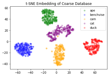
After successfully training the network, we obtain relatively good results. We visualize the feature space by passing all the data forward once to generate the features. After that, we use both PCA and t-SNE in order to visualize the data in the feature space.

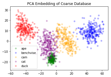(a) PCA Embedding (Synthetic)	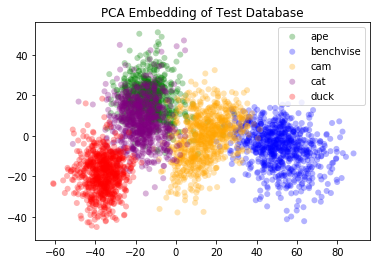(b) PCA Embedding (Real / Test Data)
(a) t-SNE Embedding (Synthetic)	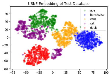(b) t-SNE Embedding (Real / Test Data)

Object Detection & 3D Pose Estimation

The custom hinge-based loss helped form the feature space to satisfy the following requirements:

$L_{triplets}$ helped objects from the same class to be “pulled” closer together and from different classes to be “pushed” far away from each other.
$L_{pairs}$ helped objects from the same class with similar pose to be “pulled” closer together. Objects with different poses (within the same class) are “pushed” away from each other.

Our loss optimizes the above two criteria simultaneously. It yields in a feature space that is semantically divided such as objects of the same class are clustered together. Objects within a class cluster are re-organized such that similar poses are closer together. This formulation allows for both object detection and 3D pose estimation using a nearest neighbour approach. An object is compared against an existing database of classes and poses. Database feature vectors are pre-computed. For each new object, a feature vector is computed using a forward pass. Afterwards, we search for the closest feature vector to the generated one in the database and predict its label and pose.

Note that, the higher number of poses per class in the dataset, the better our pose estimation is. The granularity of pose estimation is a hyperparameter inferred from industry-specifc needs.

References

[1]P. Wohlhart and V. Lepetit, “Learning descriptors for object recognition and 3d pose estimation,” in Proceedings of the IEEE Conference on Computer Vision and Pattern Recognition, 2015, pp. 3109–3118.